Cara Freeze Excel Dasar Office Belajar Microsoft Office Terbaru
Using Keyboard Shortcut ALT + W + F + F to Freeze First 3 Columns. We can use a useful keyboard shortcut to freeze columns . We can press ALT + W + F + F together to freeze columns. STEPS: To do so, first, we need to select the column next to the columns we want to freeze.
Mengenal Cara Freeze di Excel Terhadap Baris dan Kolom Data Lifestyle
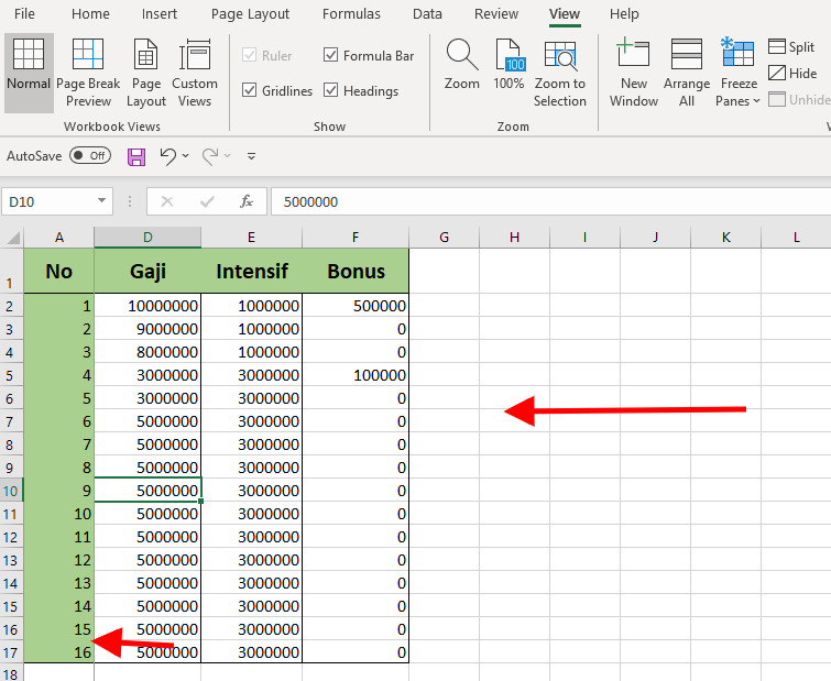
Freeze Two or More Rows in Excel. To start freezing your multiple rows, first, launch your spreadsheet with Microsoft Excel. In your spreadsheet, select the row below the rows that you want to freeze. For example, if you want to freeze the first three rows, select the fourth row. On the "View" tab, in the "Window" section, choose Freeze Panes.
cara freeze excel lebih dari satu kolom How To Use Ms Office
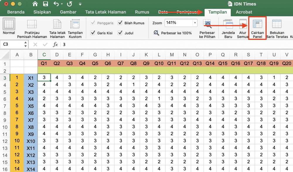
1. Freeze Kolom di Excel Kamu bisa freeze atau membekukan kolom pertama atau beberapa kolom di Excel dengan mengikuti tutorial di bawah ini: ADVERTISEMENT Cara freeze Excel kolom. Foto: Nada Shofura/kumparan Cara freeze Excel kolom. Foto: Nada Shofura/kumparan Cara freeze Excel kolom. Foto: Nada Shofura/kumparan 2. Freeze Baris di Excel
Cara Freeze Excel, Mengunci Kolom dan Baris Saat Digulir
Cara freeze excel atau mengunci kolom dan baris agar tidak bergeser saat discrol, kita bisa menggunakkan fitur freeze pains.Saat tabel atau data yang ada di.

Tutorial Cara Freeze Excel Dengan Mudah & Cepat Qwords
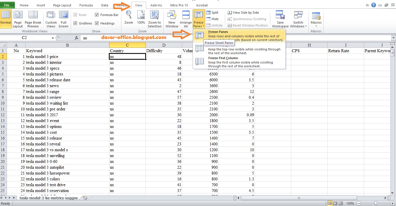
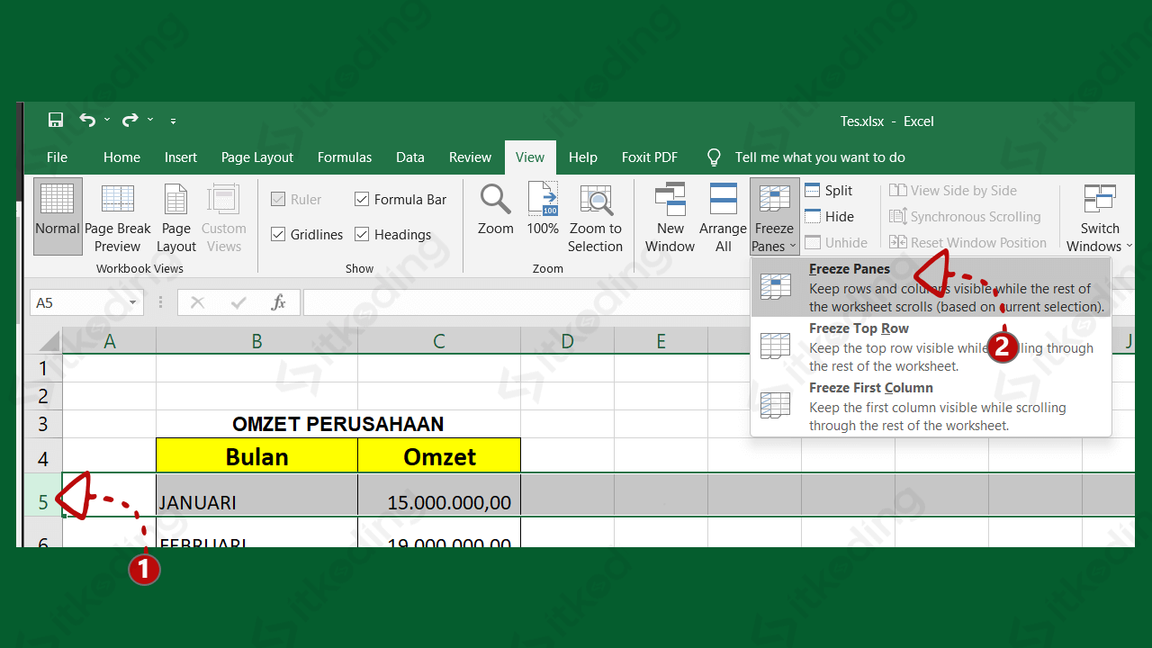
Secara universal, cara freeze excel merupakan dengan memakai menu ataupun tombol freeze. Fitur Freeze Panes ini dapat kita temukan pada Tab View- Group Window- Freeze Panes semacam yang nampak pada foto berikut. Kemudian gimana memakai fitur tersebut buat melaksanakan freeze di excel? ayo kita bahas satu persatu. 1. Cara Freeze Baris Awal Excel

√ Cara Freeze Kolom / Baris di Microsoft Excel TeknoRizen
Freeze Panes tersedia pada hampir semua versi Excel, bahkan jika kamu pengguna Office Excel 2007 dan Excel online. Penggunaan tool cara freeze Excel ini pun sama. Agar semakin mudah, berikut informasi tentang Freeze Panes yang perlu kamu tahu dan langkah-langkah penggunaannya sesuai baris atau kolom yang ingin dibekukan.

Cara Freeze Di Excel Simak Penjelasanya Ninopedia
You can freeze the first two columns by using the keyboard shortcuts: Alt + W + F + F (pressing one by one). Read More: How to Freeze First 3 Columns in Excel 2. Apply Excel Split Option to Freeze 2 Columns The Split option is a variation of Freeze Panes.
Cara Membuat Freeze Di Excel
Step 2: Remember we are not only freezing the top row, but we are freezing multiple rows at a time. Do not press ALT + W + F + R in a hurry; hold on momentarily. After selecting cell A8 under freeze panes, again select the option Freeze Panes under that. Now we can see a tiny grey straight line below the 7 th row.

Cara Freeze/Bekukan Kolom dan Baris di Microsoft Excel dengan Mudah
Secara umum, cara freeze di excel adalah dengan menggunakan menu atau tombol freeze.

Cara Mudah Freeze Kolom Pada Excel Untuk Meningkatkan Efektivitas
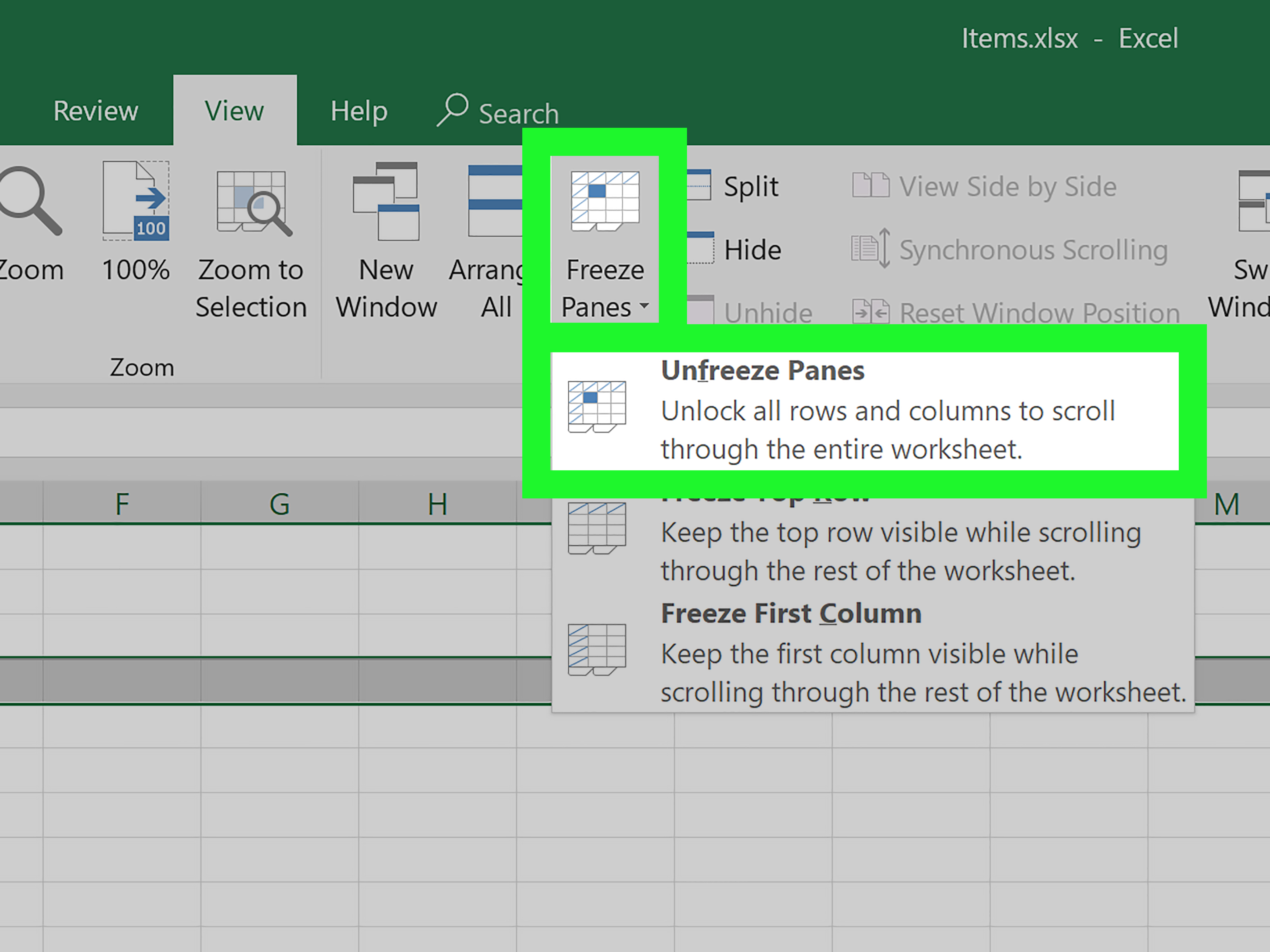
4. Select Freeze Panes and click Add. 5. Click OK. 6. To freeze the top row, select row 2 and click the magic Freeze button. 7. Scroll down to the rest of the worksheet. Result. Excel automatically adds a dark grey horizontal line to indicate that the top row is frozen. Note: to unlock all rows and columns, click the Freeze button again.
Cara Freeze Kolom dan Baris Pertama Microsoft Excel DailySocial.id
Freeze adalah fitur yang ada pada Excel yang letaknya pada menu View, gunanya untuk membekukan baris dan kolom tidak bergerak saat di scroll. Fitur ini memang sepele, tetapi kalau datanya sudah banyak maka akan berguna sekali. Freeze sendiri ada berbagai macamnya, Anda bisa membekukan bagian baris, kolom atau worksheet tertentu.
How to Freeze Cells in Excel
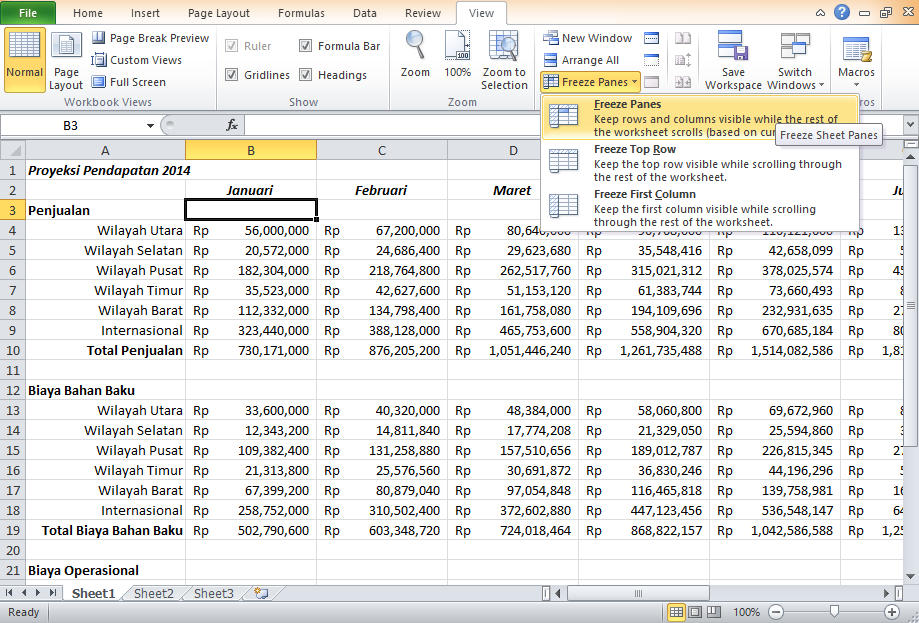
Pertama, klik cell manapun pada baris 1. Kedua, klik Tab View kemudian klik Freeze Panes Ketiga, klik Freeze Top Row kemudian silahkan scroll kebawah, dapat dipastikan posisi baris pertama ( Row 1 ) tidak berubah ketika Anda scroll seperti gambar berikut: Selanjutnya Anda silahkan lanjutkan pengisian data Anda.

Tutorial Cara Freeze Excel Dengan Mudah & Cepat Qwords
Perintah Freeze Panes digunakan untuk membekukan beberapa kolom di kiri sel yang disorot (saat scroll ke kanan atau kiri) dan beberapa baris di bagian atas sel yang disorot (saat scroll ke atas atau bawah). Pada ilustrasi di atas terbentuk 3 area yang dibekukan yaitu, Absolut freeze adalah range yang dibatasi sel terpilih dari posisi kiri atas.

Cara Freeze/Bekukan Kolom dan Baris di Microsoft Excel dengan Mudah
Langkah 1: Buka Spreadsheet Google Langkah 2: Blokir Baris atau Kolom Langkah 3: Freeze Baris atau Kolom Langkah 4: Mengubah Freeze Kelebihan Cara Freeze Excel di Google Spreadsheet 1. Memudahkan Analisis Data 2. Meningkatkan Efisiensi Kerja 3. Mempermudah Kolaborasi FAQ Mengenai Freeze Excel di Google Spreadsheet 1.

Cara Freeze/Bekukan Kolom dan Baris di Microsoft Excel dengan Mudah
Langkah pertama yang perlu Anda lakukan adalah membuka file excel yang ingin dicetak. Setelah itu, pilih lembar kerja yang ingin Anda freeze. Kemudian, lihatlah menu bar di atas layar Anda dan cari opsi "View" atau "Tampilan". Di dalam opsi tersebut, Anda akan menemukan "Freeze Panes" atau "Freeze Lembar Kerja".

Cara Freeze Excel Kunci Kolom dan Baris di Excel YouTube
Select View > Freeze Panes > Freeze First Column. The faint line that appears between Column A and B shows that the first column is frozen. Freeze the first two columns. Select the third column. Select View > Freeze Panes > Freeze Panes. Freeze columns and rows. Select the cell below the rows and to the right of the columns you want to keep.